Weighted Graphs
Weighted graphs are an alternative universe of problems than unweighted graphs. If we're traveling to California, we don't just care about the number of roads traveled on. The edges of road networks are naturally bound to numerical values such as construction cost, traversal time, length, or speed limit. Identifying the shortest path in such graphs proves more complicated than breadth-first search in unweighted graphs, but opens the door to a wide range of applications.
Information on this page comes from The Algorithm Design Manual by Skiena.
Minimum Spanning Trees
A spanning tree of a graph \(G = (V, E)\) is a subset of edges from \(E\) forming a tree connecting all vertices of \(V\). For edge-weighted graphs, we are particularly interested in the minimum spanning tree - the spanning tree whose sum of edge weights is as small as possible. Minimum spanning trees are the answer whenever we need to connect a set of points (representing cities, homes, junctions, or other locations) by the smallest amount of roadway, wire, or pipe. Minimum spanning trees are also useful for clustering.
There can be more than one minimum spanning tree in a graph. Indeed, all spanning trees of an unweighed (or equally weighted) graph \(G\) are minimum spanning trees, since each contains exactly \(n - 1\) equal-weight edges. Such a spanning tree can be found using depth-first or breadth-first search. Finding a minimum spanning tree is more difficult for general weighted graphs, however two different algorithms are presented below.
Prim's Algorithm
Prim's algorithm for minimum spanning trees starts from one vertex and grows the rest of the tree one edge at a time until all vertices are included. Greedy algorithms make the decision of what to do next by selecting the best local option from all available choices without regard to the global structure. Since we week the tree of minimum weight, the natural greedy algorithm for a minimum spanning tree repeatedly selects the smallest weight edge that will enlarge the number of vertices in the tree. Prim's algorithm can be implemented as \(O(m + n\lg{n})\) with a priority-queue.
prim-mst(G)
    select an arbitrary vertex s to start the tree from
    while (there are still non tree vertices)
        select the edge of minimum weight between a tree and non tree vertex
        add the selected edge and vertex to the tree T_prim
The correctness of this algorithm can be proven by contradiction. We assert that there must be a specific instant where the tree went wrong. However, since we always select the smallest edge, it's not possible for a smaller edge to exist than the one we're adding (otherwise it would have already been chosen).
Kruskal's Algorithm
Kruskal's algorithm is an alternative approach to finding minimum spanning trees that proves more efficient on sparse graphs. Like Prim's, Kruskal's algorithm is greedy. Unlike Prim's, it does not start with a particular vertex. Kruskal's algorithm builds up connected components of vertices, culminating in a minimum spanning tree. Initially, each vertex forms its own separate component in the tree-to-be. The algorithm repeatedly considers the lightest remaining edge and tests whether its two endpoints lie within the same connected component. If so, this edge will be discarded, because adding it would create a cycle in the tree-to-be. If the endpoints are in different components, we insert the edge and merge the two components into one. Since each connected component is always a tree, we need never explicitly test for cycles.
kruskal-mst(g)
    put the edges in a priority queue ordered by weight
    count = 0
    while (count < n - 1) do
        get next edge (v, w)
        if (component(v) != component(w))
            add to T_kruskal
            merge component(v) and component(w)
The speed of Kruskal's algorithm depends on the component test. This test may be implemented by a breadth-first or depth-first search in a sparse graph. With this approach, Kruskal's algorithm is \(O(mn)\). However, a faster implementation exists with the union-find data structure.
The Union-Find Data Structure
A set partition is a partitioning of the elements of some universal set (say the integers 1 to \(n\)) into a collection of disjointed subsets. Thus each element must be in exactly one subset. Set partitions naturally arise in graph problems such as connected components (each vertex is in exactly one connected component) and vertex coloring (a person may be male or female, but not both or neither).
The connected components in a graph can be represented as a set partition. For Kruskal's algorithm to run efficiently, we need a data structure that efficiently supports the following operations:
- \(same\ component(v_1, v_2)\)
- \(merge\ component(C_1, C_2)\)
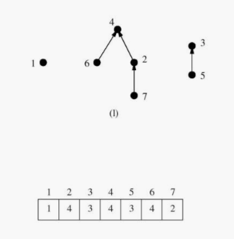
The union find data structure represents each subset as a "backwards" tree with pointers from a node to its parent. Each node of this tree contains a set element, and the name of the set is taken from the key at the root.
We implement our desired component operations in terms of two simpler operations, union and find:
find(i)- Find the root of the tree containing element
i, by walking up the pointers until there is nowhere to go. Return the label of the root.
- Find the root of the tree containing element
union(i, j)- Link the root of one of the trees (say containing
i) to the root of the tree containing the other (sayj) sofind(i)now equalsfind(j).
- Link the root of one of the trees (say containing
Tree structures can be very unbalanced, so we must limit the height of our
trees. The most obvious means of control is the decision of which of the two
component roots becomes the root of the combined component on each
union. To minimize the tree height, it is of course better to make the
smaller tree the subtree of the bigger one.
With union-set, we can do both unions and finds in \(O(\log{n})\).
Shortest Paths
A path is a sequence of edges connecting two vertices. The shortest path from \(s\) to \(t\) in an unweighted graph can be constructed using a breadth-first search from \(s\). The minimum-link path is recorded in the breadth-first search tree, and it provides the shortest path when all edges have equal weight. However, BFS does not suffice to find shortest paths in weighted graphs. The shortest weighted path might use a large number of edges.
Finding the shortest path between two nodes in a graph arises in many different applications. These may include transportation problems and computer network communication problems. Many applications reduce to the finding shortest path, learn to smell this! Page 212 of The Algorithm Design Manual contains a lovely example (Dialing for Documents).
Dijkstra's Algorithm
Dijkstra's algorithm is the method of choice for finding shortest paths in an edge-and/or vertex-weighted graph. Given a particular start vertex \(s\), it finds the shortest path from \(s\) to every other vertex in the graph including your desired destination \(t\).
Suppose the shortest path from \(s\) to \(t\) in graph \(G\) passes through a particular intermediate vertex \(x\). Clearly, this path must contain the shortest path from \(s\) to \(x\) as its prefix, because if not, we could shorten our \(s\) to \(t\) path by using a shorter \(s\) to \(x\) prefix. Thus, we must compute the smallest path from \(s\) to \(x\) before we find the path from \(s\) to \(t\).
Dijkstra's algorithm proceeds in a series of rounds, where each round establishes the shortest path from \(s\) to some new vertex. Specifically, \(x\) is the vertex that minimizes \(dist(s, v_i) + w(v_i, x)\) over all finished \(1 \leq i \leq n\), where \(w(i, j)\) is the length of the edge from \(i\) to \(j\), and \(dist(i, j)\) is the length of the shortest path between them.
import math

def dijkstra(graph, s, t):
    known = {s}
    distances = {vertex: math.inf for vertex in graph.all_vertices()}
    for neighbor in s.get_neighbors():
        distances[neighbor] = weight(s, neighbor)
    last = s
    while last != t:
        v_next = min(distances[v] for v in (graph.all_vertices() - known))
        for neighbor in v_next.get_neighbors():
            distances[neighbor] = min(distances[neighbor],
                                      distances[v_next] + weight(v_next, neighbor))
        last = v_next
        known.add(v_next)
The basic idea is very similar to Prim's algorithm. In each iteration, we add exactly one vertex to the tree of vertices for which we know the shortest path from \(s\). The difference between Dijkstra's and Prim's algorithm is how they rate the desirability of each outside vertex. In the minimum spanning tree problem, all we cared about was the weight of the next potential tree edge. In shortest path, we want to include the closest outside vertex o(in shortest-path distance) to \(s\). This is a function of both the new edge weight and the distance from \(s\) to the tree vertex it is adjacent to.
All-Pairs Shortest Path
Sometimes we want to find the shortest path between all pairs of vertices in a given graph. We could solve the all-pairs shortest path by calling Dijkstra's algorithm from each of the \(n\) possible starting vertices (\(O(n^3)\)). But Floyd's all-pairs shortest-path algorithm is a slick way to construct an \(n x n\) distance matrix from the original weight matrix of the graph. This algorithm is also \(O(n^3)\), but the loops are so tight and the program so short that it runs better in practice.
Floyd's algorithm starts with the adjacency matrix. The edge \((i, j)\) should have its weight in matrix[i][j]. Cells for which the edge doesn't exist should be set to MAXINT.
def floyd(adjacency_matrix):
    n_vertices = len(adjacency_matrix)
    for k in range(n_vertices):
        for i in range(n_vertices):
            for j in range(n_vertices):
                through_k = adjacency_matrix[x][k] + adjacency_matrix[k][y]
                if (through_k < adjacency_matrix[x][y]):
                    adjacency_matrix[x][y] = through_k
We define \(W[i, j]^k\) to be the length of the shortest path from \(i\) to \(j\) using only vertices numbered from 1, 2, …, \(k\) as possible intermediate vertices. At each iteration, we allow a richer set of possible shortest paths by adding a new vertex as a possible intermediary. Allowing the $k$th vertex as a stop helps only if there is a short path that goes through \(k\), so \(W[i, j]^k = min(W[i, j]^{k - 1}, W[i, k]^{k - 1}, + W[k, j]^{k - 1})\).