Graphs
A graph \(G = (V, E)\) consists of a set of vertices \(V\) together with a set \(E\) of vertex pairs or edges. Graphs can represent essentially any relationship. The key to using graph algorithms effectively in applications often lies in correctly modeling your problem so you can take advantage of existing algorithms.
Also see weighted graphs.
Note: This page comes from Algorithms by Dasgupta et al. and The Algorithm Design Manual by Skiena.
Overview
Formally, a graph is specified by a set of vertices (also called nodes) \(V\) and by edges \(E\) between select pairs of vertices. In the example below, \(V = \{1, 2, 3, 4, 5, 6\}\) and \(E = \{\{1, 1\}, \{1, 2\}, \{1, 4\}, \{2, 4\}, \{2, 5\}, \{3, 5\}, \{4, 6\}\}\).
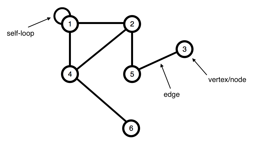
An edge means that "x is connected with y." This is a symmetric relation - it implies also that y is connected with x - and we denote it using set notation, \(e = \{x, y\}\). Such edges are undirected and are part of an undirected graph.
Sometimes graphs depict relations that do not have this reciprocity, in which case it is necessary to use edges with directions on them. There can be directed edges \(e\) from x to y (written \(e = (x, y)\)), or both. Directed graphs contain directed edges. Directed edges are drawn with arrows on them.
Flavors of Graphs
Several fundamental properties of graphs impact the choice of the data structures used to represent them and algorithms available to analyze them.
- Undirected vs. Directed
- A graph \(G = (V, E)\) is undirected if edge \((x, y) \in E\) implies that \((y, x) \in E\). If not, we say that the graph is directed.
- Weighted vs. Unweighted
- Each edge (or vertex) in a weighted graph \(G\) is assigned a numerical value, or weight. In unweighted graphs, there is no cost distinction between various edges and vertices.
- The difference between weighted and unweighted graphs becomes particularly apparent in finding the shortest path between two vertices.
- Simple vs. Non-simple
- Any graph that avoids self-loops and multiedges is called simple. A self-loop is an edge \((x, x)\) involving only one vertex. An edge \((x, y)\) is a multiedge if it occurs more than once in the graph.
- Sparse vs. Dense
- Graphs are sparse when only a small fraction of the possible vertex pairs actually have edges defined between them. Graphs where a large fraction of the vertex pairs define edges are called dense.
- The degree of a vertex is the number of edges adjacent to it.
- In a regular graph, each vertex has exactly the same degree.
- Cyclic vs. Acyclic
- An acyclic graph does not contain any cycles.
- Trees are connected, acyclic undirected graphs.
- Embedded vs. Topological
- A graph is embedded if the vertices and edges are assigned geometric positions.
- Implicit vs. Explicit
- Certain graphs are not explicitly constructed and then traversed, but built as we use them.
- Labeled vs. Unlabeled
- Each vertex is assigned a unique name or identifier in a labeled graph to distinguish it from all other vertices. In unlabeled graphs, no such distinctions have been made.
Social networks are graphs where the vertices are people, and there is an edge between two people if and only if they are friends.
Representations
The two basic graph data structures are adjacency matrices and adjacency lists. We assume a graph \(G = (V, E)\) contains \(n\) vertices and \(m\) edges. Adjacency lists are the right data structure for most applications of graphs.
Adjacency Matrix
We can represent a graph by an adjacency matrix; if there are \(n = |V|\) vertices \(v_1,...,v_n\), this is an \(nxn\) array whose \((i, j)\) th entry is:
\begin{equation} a_{ij} = \begin{cases} \text{1} &\quad\text{if there is an edge from $v_i$ to $v_j$}\\ \text{0} &\quad\text{otherwise.} \ \end{cases} \end{equation}For undirected graphs, the matrix is symmetric since an edge \(\{u, v\}\) can be taken in either direction.
Here's the adjacency matrix for the graph above:
| 1 | 1 | 0 | 1 | 0 | 0 |
| 1 | 0 | 0 | 1 | 1 | 0 |
| 0 | 0 | 0 | 0 | 1 | 0 |
| 1 | 1 | 0 | 0 | 0 | 1 |
| 0 | 1 | 1 | 0 | 0 | 0 |
| 0 | 0 | 0 | 1 | 0 | 0 |
The biggest convenience of this format is that the presence of a particular edge can be checked in constant time, with just one memory access. On the other hand the matrix takes up \(O(|V|^2)\) space, which is wasteful if the graph does not have very many edges.
Adjacency List
An alternative representation to the adjacency matrix, with size proportional to the number of edges, is the adjacency list. It consists of \(|V|\) linked lists, one per vertex. The linked list for vertex \(u\) holds the names of vertices to which \(u\) has an outgoing edge - that is, vertices \(v\) for which \((u, v) \in E\). Therefore, each edge appears in exactly one of the linked lists if the graph is directed or two of the lists if the graph is undirected. Either way, the total size of the data structure is \(O(|E|)\). Checking for a particular edge \((u, v)\) is no longer constant time, because it requires sifting through \(u\)'s adjacency list. But it is easy to iterate through all neighbors of a vertex (by running down the corresponding linked list), and, as we shall soon see, this turns out to be a very useful operation in graph algorithms. Again, for undirected graphs, this representation has a symmetry of sorts: \(v\) is in \(u\)'s adjacency list if and only if \(u\) is in \(v\)'s adjacency list.
Adjacency Matrix vs. Adjacency List
Which of the two representations is better? Well, it depends on the relationship between \(|V|\), the number of nodes in the graph, and \(|E|\), the number of edges. \(|E|\) can be as small as \(|V|\) (if it gets much smaller, then the graph degenerates - for example, has isolated vertices), or as large as \(|V|^2\) (when all possible edges are present). When \(|E|\) is close to the upper limit of this range, we call the graph dense. At the other extreme, if \(|E|\) is close to \(|V|\), the graph is sparse. Exactly where \(|E|\) lies in this range is usually a crucial factor in selecting the right graph algorithm.
Traversal
The key idea behind graph traversal is to mark each vertex when we first visit it and keep track of what we have not yet completely explored. Each vertex may be undiscovered, discovered, or processed. We must maintain a structure containing the vertices that we have discovered but not yet completely processed.
Breadth-First Search (BFS)
The basic breadth-first search algorithm is given below. The algorithm explores wide before going deep; we look at each child before looking at any of the children's children. BFS takes \(O(n + m)\) time.
def bfs(graph, root):
    parent = {}
    discovered = {root}
    queue = [root]
    while queue:
        current = queue.pop(0)
        for neighbor in get_adjacent(current, graph):
            if neighbor not in discovered:
                parent[neighbor] = current
                discovered.add(neighbor)
                queue.append(neighbor)
Note that to search an entire graph one would need to apply this function to each vertex in the graph.
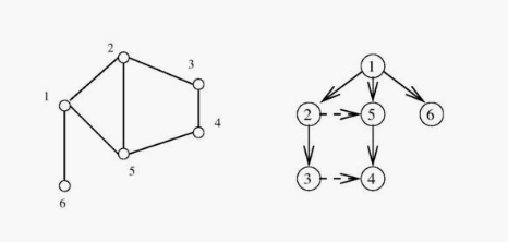
In this implementation of breadth-first search, we assign a direction to each
edge, from the discoverer current to the discovered neighbor. We maintain
a parent map which defines a tree on the vertices of the graph. This tree
contains the shortest path from the root to every other node in the tree. A
breadth-first search tree can be seen in the right of the image below.
The graph edges that do not appear in the breadth-first search tree also have special properties. For undirected graphs, non-tree edges can point only to vertices on the same level as the parent vertex, or to vertices on the level directly below the parent. These properties follow easily from the fact that each path in the tree must be the shortest path in the graph.
Applications of BFS
- Connected Components
A connected component of an undirected graph is a maximal set of vertices such that there is a path between every pair of vertices. The components are separate "pieces" of the graph such that there is no connection between the pieces. An amazing number of seemingly complicated problems reduce to finding or counting connected components. For example, testing whether a puzzle such as the Rubik's Cube or the 15 puzzle can be solved from any position is really asking whether the graph of legal configurations is connected.
Connected components can be found using breadth-first search since vertex order does not matter. We start from the first vertex. Anything we discover during this search must be part of the same connected component. We then repeat the search from any undiscovered vertex (if one exists) to define the next component, and so on until all vertices have been found.
- Two-Coloring Graphs
The vertex-coloring problem seeks to assign a label (or color) to each vertex of a graph such that no edge links any two vertices of the same color. We can easily avoid all conflicts by assigning each vertex a unique color. However, the goal is to use as few colors as possible.
A graph is bipartite if it can be colored without conflicts while using only two colors. Consider the "had-sex-with" graph in a heterosexual world. Men have sex only with women, and vice versa. Thus gender defines a legal two-coloring, in this simple model.
We can augment breadth-first search so that whenever we discover a new vertex, we color it the opposite of its parent. We check whether any nondiscovery edge links two vertices of the same color. Such a conflict means that the graph cannot be two-colored.
Depth-First Search (DFS)
The difference between BFS and DFS results is in the order in which they explore vertices. This order depends completely upon the container data structure used to store the unprocessed vertices: BFS uses a queue, DFS uses a stack. DFS implementations often use recursion instead of an explicit stack. Depth-first search explores deep before going wide; the algorithm looks at the entirety of a child before moving to the next child.
def dfs(root, graph):
    discovered = set()
    parent = {}

    def search(node):
        discovered.add(node)
        for neighbor in get_adjacent(node, graph):
            if neighbor not in discovered:
                parent[neighbor] = root
                dfs(neighbor, graph)

    search(root)
Note that some implementations of depth-first search also maintain the
traversal time for each vertex. A time clock ticks each time we enter or
exit any vertex. entry_time and exit_time dictionaries go from node ->
time. The time intervals can tell us a vertex's ancestor and how many
descendants it has.
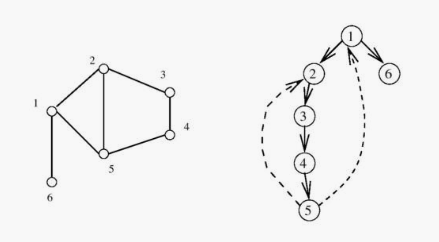
Depth-first search partitions the edges of an undirected graph into exactly
two classes: tree edges and back edges. The tree edges discover new
vertices, and are those encoding in the parent relation (seen in the image
above). Back edges are those whose other endpoint is an ancestor of the
vertex being expanded, so they point back into the tree.
Applications of DFS
- Finding Cycles
Back edges are the key to finding a cycle in an undirected graph. If there is no back edge, all edges are tree edges, and no cycle exists in a tree. But any back edge going from \(x\) to an ancestor \(y\) creates a cycle with the tree path from \(y\) to \(x\).
def has_cycle(node, graph, discovered=None): if discovered is None: discovered = set() discovered.add(node) return any((neighbor in discovered or has_cycle(graph, neighbor, discoverd)) for neighbor in get_adjacent(node, graph)) - Articulation Vertices
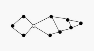
The articulation vertex is a single vertex whose deletion disconnects a connected component of the graph. Any graph that contains an articulation vertex is inherently fragile, because deleting that single vertex causes a loss of connectivity between other nodes. The connectivity of a graph is the smallest number of vertices whose deletion will disconnect the graph. The connectivity is one if the graph has an articulation vertex. More robust graphs without such a vertex are said to be biconnected.
Testing for articulation vertices by brute force is easy. Temporarily delete each vertex \(v\), and then do a BFS or DFS traversal of the remaining graph to establish whether it is still connected. The total time is \(O(n(m + n))\).
DFS gives a clever, linear-time algorithm. Look at the depth-first search tree. If this tree represents the entirety of the graph, all internal (non-leaf) nodes would be articulation vertices, since deleting any one of them would separate a leaf from the root. A depth-first search of a general graph partitions the edges into tree edges and back edges. Think of these back edges as security cables linking a vertex back to one of its ancestors. Finding articulation vertices requires maintaining the extent to which back edges (i.e. security cables) link chunks of the DFS tree back to ancestor nodes.
DFS on Directed Graphs
When traversing undirected graphs, every edge is either in the depth-first search tree or a back edge to an ancestor in the tree. For directed graphs, depth-first search labelings can take on a wider range of possibilities: tree edges, forward edges, back edges, and cross edges.
- Topological Sorting
Topological sorting is the most important operation on directed acyclic graphs (DAGs). It orders the vertices on a line such that all directed edges go from left to right. Such an ordering cannot exist if the graph contains a directed cycle, because there is no way you can keep going from right on a line and still return back to where you started from!
Each DAG has at least one topological sort. The importance of topological sorting is that it gives us an ordering to process each vertex before any of its successors. For example, suppose college courses are vertices and prerequisites are edges. Your transcript is a topological sort of courses.
Topological sorting can be performed efficiently using depth-first searching. A directed graph is a DAG if and only if no back edges are encountered. Labeling the vertices in the reverse order that they are marked processed finds a topological sort of a DAG (i.e. record when you finish processing then reverse the collection).
TODO Glossary of Terms
Taken from Algorithms by Sedgewick and Wayne. See http://algs4.cs.princeton.edu/41graph/
- A self-loop is an adge that connects a vertex to itself.
- When an edge connects two vertices, we say that the vertices are adjacent to one another and that the edge is incident on both vertices.
- The degree of a vertex is the number of edges incident to it.
- A path in a graph is a sequence of vertices connected by edges.
- A cycle is a path (with at least one edge) whose first and last vertices are the same.
- We say that one vertex is connected to another if there exists a path that contains both of them.
- A graph is connected if there is a path from every vertex to every other vertex.
- An acyclic graph is a graph with no cycles.
- A tree is a acyclic connected graph.
- A forest is a disjoint set of trees.