Dynamic Programming

Let's look at a simple program for computing the nth Fibonacci number.

def fib(n):
    if n == 0:
        return 0
    if n == 1:
        return 1
    return fib(n - 1) + fib(n - 2)

The course of execution for this recursive algorithm is illustrated by its recursion tree.

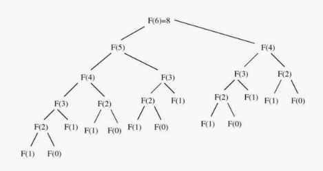
Note that \(F(4)\) is computed on both sides of the recursion tree, and \(F(2)\) is computed no less than five times in this small example. This redundancy drastically affects performance.

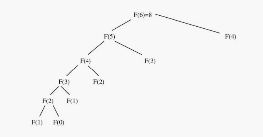
We can improve performance by storing (or caching) the results of each Fibonacci computation \(F(k)\) indexed by the parameter \(k\).

cache = {0: 0, 1: 1}
def fib(n):
    if n not in cache:
        cache[n] = fib(n - 1) + fib(n - 2)
    return cache[n]

This approach is a simple way to get most of the benefits of full dynamic programming. Here's the recursion tree:

Let's go a step further with full dynamic programming! We can calculate \(F(n)\) in linear time and space with no recursive calls by explicitly specifying the order of evaluation of the recurrence relation.

def fib(n):
    f = [0, 1]
    for i in range(2, n + 1):
        f.append(f[i - 1] + f[i - 2])
    return f[n]

However, more careful study shows that we do not need to store all the intermediate values for the entire period of execution.

def fib(n):
    if n == 0:
        return 0

    back_2, back_1 = 0, 1
    for _ in range(2, n):
        back_2, back_1 = back_1, back_1 + back_2
    return back_1 + back_2

This analysis reduces the storage demands to constant space with no asymptotic degradation in running time.

To deal with inexact string matching, we must first define a cost function telling us how far apart two strings are - i.e., a distance measure between pairs of strings. Edit distance reflects the number of changes that must be made to convert one string to another. There are three natural types of changes: substitution, insertion, and deletion. Edit distance assigns each operation an equal cost of 1. Here's a recursive edit distance function:

def edit_distance(source, target):
    if not source:
        return len(target)
    if not target:
        return len(source)

    substitution_cost = 0 if source[-1] == target[-1] else 1
    return min(edit_distance(source[:-1], target[:-1]) + substitution_cost,
               edit_distance(source, target[:-1]) + 1,  # insertion
               edit_distance(source[:-1], target) + 1)  # deletion

This program is absolutely correct but impossible slow. A table-based, dynamic programming implementation of this algorithm is given below. costs is a two-dimensional matrix where each cell contains the optimal solution to a subproblem (i.e. costs[x][y] is edit_distance(source[:x], target[:y])).

def edit_distance(source, target):
    costs = [[None for _ in range(len(target) + 1)]
             for _ in range(len(source) + 1)]

    for index in range(len(costs)):
        costs[index][0] = index
    for index in range(len(costs[0])):
        costs[0][index] = index

    for x in range(1, len(source) + 1):
        for y in range(1, len(target) + 1):
            substitution_cost = 0 if source[x - 1] == target[y - 1] else 1
            costs[x][y] = min(costs[x - 1][y - 1] + substitution_cost,
                              costs[x - 1][y] + 1,  # insertion
                              costs[x][y - 1] + 1)  # deletion
    return costs[-1][-1]

The first row and the first column represent the empty prefix of the source and target, respectively. This is why the matrix height/width is larger than the source/target length.

Note that it is unnecessary to store the entire O(mn) matrix. The recurrence only requires two rows at a time. Thus, this algorithm could be further optimized to O(n) space without changing the time complexity.

Here is a more sophisticated application of dynamic programming. Consider the problem of finding the maximum sum over all subarrays of a given array of integers. For example, the following array's max subarray starts at index 0 and ends at index 3.

[904, 40, 523, 12, -335, -385, -124, 481, -31]

The brute-force algorithm, which computes each subarray sum, has \(O(n^3)\) time complexity.

Here's a solution with dynamic programming. The maximum subarray must end at some position. Notice that the largest range ending at \(i\) is best_at(i) = max(A[i], A[i] + best_at(i - 1)). Our final answer is the maximum "best_at" over all i. Here's an approach with memoization.

def max_subarray(array):
    cache = {}

    def best_at(array, index):
        if index not in cache:
            if index == 0:
                cache[0] = array[0]
            else:
                cache[index] = max(array[index], cache[index - 1] + array[index])
        return cache[index]

    return max(best_at(array, index) for index in range(len(array)))

Let's remove the recursive calls and use dynamic programming.

def max_subarray(array):
    best_at = [None] * len(array)
    for index in array:
        if index == 0:
            best_at[index] = array[index]
        else:
            best_at[index] = max(array[index], array[index] + best_at[index - 1])
    return max(best_at)

Finally, notice that we can go to constant space by only remembering the last "best_at" and the maximum.

def max_subarray(array):
    last, best = array[0], array[0]
    for index in range(1, len(array)):
        last = max(array[index], last + array[index])
        best = max(last, best)
    return best

There are three steps involved in solving a problem by dynamic programming:

1. Formulate the answer as a recurrence relation or recursive algorithm.
2. Show that the number of different parameter values taken on by your recurrence is bounded by a (hopefully small) polynomial.
3. Specify an order of evaluation for the recurrence so the partial results you need are always available when you need them.

In practice, you'll find that dynamic programming algorithms are usually easier to work out from scratch than look up.

Suppose three workers are given the task of scanning through a shelf of books in search of a given piece of information. To get the job done fairly and efficiently, the books are to be partitioned among the three workers. If the books are the same length, the job is easy: 100 100 100 | 100 100 100 | 100 100 100. If the books are not the same length, the task becomes more difficult (100 200 300 400 500 | 600 700 | 800 900). An algorithm that solves this linear partition problem takes as input an arrangement \(S\) of nonnegative numbers and an integer \(k\). The algorithm should partition \(S\) into \(k\) or fewer ranges, to minimize the maximum sum over all ranges, without reordering any of the numbers.

A heuristic to solve this problem might compute the average size of a partition and then try and insert dividers to come close to this average. Unfortunately, this method is doomed to fail on certain inputs.

Instead, consider a recursive, exhaustive search approach to solving this problem. The /k/th partition starts right after we placed the (k - 1)st divider. Where can we place this last ((k - 1)st) divider? Between the ith and (i + 1)st elements for some \(i\), where \(1 \leq i \leq n\). What is the cost of this? The total cost will be the larger of two qualtities - (1) the cost of the last partition and (2) the cost of the largest partition formed to the left of \(i\). What is the size of this left partition? To minimize our total, we want to use the \(k - 2\) remaining dividers to partition the elements \(\{s_1, ..., s_i\}\) as equally as possible. This is a smaller instance of the same problem and hence can be solved recursively!

Therefore, let us define \(M[n, k]\) to be the minimum possible cost over all partitions of \(\{s_1, ..., s_n\}\) into \(k\) ranges, where the cost of a partition is the largest sum of elements in one of its parts. Thus defined, this function cab be evaluated:

This recurrence can be solved with dynamic programming in \(O(kn^2)\) time. Note that we also need a second matrix, \(D\) to reconstruct the optimal partition. Whenever we update the value of \(M[i, j]\), we record which divider position was required to achieve that value.

See ../theory/cfg.html.