Trees

Overview

A tree is an acyclic, connected graph. In other words, any two vertices are connected by exactly one path. Conventional tree operations are insert, search, remove, and traverse.

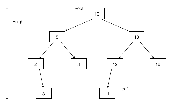
The root indicates the top of the tree.
Leaves refer to nodes with no children.
A parent is the node above the current one. A child is the node below the current one.
The depth of a node n is the number of nodes on the search path from root to n, not including /n itself.
The height of a tree is the maximum depth of any node.
A level of a tree is all nodes at the same depth.
A node is an ancestor of d if it lies on the search path from the root to d. If a node is an ancestor of d, we say d is a descendant of that node.
A tree is balanced when every path from root to leaf has the same length.

Binary Search Tree

A binary tree is recursively defined as being empty or consisting of a root node with left and right subtrees. A binary search tree (BST) labels each node in a binary tree with a single key such that for any node labeled \(x\), all nodes in the left subtree have \(keys < x\) while all nodes in the right subtree have \(keys > x\).

∀ y ∈ left subtree of x, y ≤ x
∀ y ∈ right subtree of x, y ≥ x

Binary tree nodes have left and right pointer fields, an optional parent pointer, and a data field.

from collections import namedtuple

Node = namedtuple("Node", ["left", "right", "data"])

Binary search trees can be used to solve almost every data structures problem reasonably efficiently. They offer the ability to efficiently search for a key as well as find the min and max elements, look for the successor or predecessor of a search key, and enumerate the keys in a range in sorted order.

Traversal

Traversal involves visiting all nodes. In-order traversal of a binary search tree can be done recursively with the following.

def traverse(tree):
    if tree:
        traverse(tree.left)
        process(tree.item)
        traverse(tree.right)

Changing the position of process gives alternate traversal orders. Processing the item first yields a pre-order traversal, while processing it last gives a post-order traversal.

Performance

Search, insert, and delete all take \(O(h)\) time, where \(h\) is the height of the tree. A perfectly balanced tree has \(h = \lceil \log n \rceil\). Unfortunately, inserting keys in sorted order produces a skinny linear height tree, \(h = n\). Randomizing insert order will produce \(O(\log n)\) height on average.

Operation	Best Complexity	Worst Complexity
Insert	\(O(\log n)\)	\(O(n)\)
Search	\(O(\log n)\)	\(O(n)\)
Delete	\(O(\log n)\)	\(O(n)\)

A binary search tree is complete if every node has zero or two children and all leaves are at the same level.

Balanced Search Trees

Balanced binary search tree data structures adjust the tree during insertion/delete to guarantee that height will always be \(O(\log n)\). Balanced tree implementations include red-black trees and splay trees.