Coursera: Machine Learning
Week 1
Introduction
What is Machine Learning?
"A computer program is said to learn from experience E with respect to some task T and some performance measure P, if its performance on T as measured by P, improves with experience E." Tom Mitchell
In general, any machine learning can be assigned to one of two broad classifications: supervised learning and unsupervised learning. But other types include reinforcement learning and recommender learning.
Supervised Learning
The algorithm in supervised learning receives a dataset where the "right answers" for each example is included. We know what the correct output should look like, having the idea that there is a relationship between the input and the output.
Supervised learning problems are classified into regression and classification problems. In a regression problem we try and find a continuous valued output. We map input variables to some continuous function. In contrast, a classification problem produces discrete valued output. We are trying to map input variables into discrete categories. TODO: Features
Unsupervised Learning
Unsupervised learning tries to find structure in a dataset where we have no idea what the results should look like. Clustering is an example of unsupervised learning. The "Cocktail Party Algorithm" is another; it allows you to find structure in a chaotic environment. (i.e. identifying individual voices and music from a mesh of sounds at a cocktail party).
Linear Regression with One Variable
Model Representation
In this course, we'll use \(x^{(i)}\) to denote the "input" variables or features and \(y^{(i)}\) to denote the "output" or target variable. A pair \((x^{(i)}, y^{(i)})\) is called a training example, and the dataset that we'll be using to learn - a list of m training examples \((x^{(i)}, y^{(i)}); i = 1,...,m\) - is called a training set. We will also use \(X\) to denote the space of input values, and \(Y\) to denote the space of output values. In this example, \(X = Y = ℝ\).
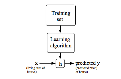
To describe the supervised learning problem slightly more formally, our goal is, given a training set, to learn a function h: X -> Y so that h(x) is a "good" predictor for the corresponding value of y. For historical reasons, this function h is called a hypothesis.
Cost Function
For linear regression of one variable, we use the hypothesis function \(h_\theta(x_i) = \theta_0 + \theta_1 x^{(i)}\). We can measure the accuracy of our hypothesis function by using a cost function. This (effectively) takes an average difference of all the results of the hypothesis with inputs from x's and the actual output y's.
\begin{equation} J(\theta_0, \theta_1) = \frac{1}{2m} \sum_{i=1}^{m} (h_\theta(x_i) - y_i)^2 \end{equation}This particular function \(J(\theta_0, \theta_1)\) is called the "square error function", or "mean squared error." Our goal is to
\begin{equation} \underset{\theta_0, \theta_1}{\text{minimize}}\quad J(\theta_0, \theta_1) \end{equation}i.e. to choose the value of \(\theta_0\) and \(]\theta_1\) that minimizes \(J(\theta_0, \theta_1)\). If we try to think of it in visual terms, our training data set is scattered on the x-y plane. We are trying to make a the best possible straight line which passes through these scattered data points.
Three-dimensional plots can be visualized with contour plots. Imagine these as if the color shows the height of the third-dimension.
Parameter Learning - Gradient Descent
Gradient descent allows one to estimate the parameters in a hypothesis function. It's an algorithm that allows one to find
\begin{equation} \underset{\theta_0, \theta_1}{\text{min}}\quad J(\theta_0, \theta_1) \end{equation}In addition to the hypothesis function of linear regression with one variable, gradient descent also applies to functions with more than two features.
Repeat until convergence:
\begin{equation} \theta_j := \theta_j - \alpha \frac{\partial}{\partial\theta_j} J(\theta_0, \theta_1) \end{equation}The \(:=\) operation is assignment. \(j=0,1\) represents the feature index number. This means that we simultaneously apply the assignment to each parameter. \(\alpha\) is the learning rate and it controls how big of a step we take. We take the partial derivative of our cost function gives us the direction to move toward.
Note that different starting points may end up with different results.
At the local minimum the slop (and thus the derivative) becomes zero. As a result, the assignment doesn't change the parameter and gradient descent converges. As we approach a local minimum, gradient descent will automatically take smaller steps. So no need to decrease \(\alpha\) over time.
\(\alpha\) must be chosen carefully. If \(\alpha\) is too small, gradient descent can be slow. If \(\alpha\) is too large, gradient descent can overshoot the minimum. It may fail to converge, or even diverge.
- Gradient Descent for Linear Regression
We can plug the cost function we used for linear regression into the gradient descent algorithm.
Repeat until convergence:
\begin{equation} \theta_j := \theta_j - \alpha \frac{\partial}{\partial\theta_j} \frac{1}{2m} \sum_{i=1}^{m} (h_\theta(x^{(i)}) - y^{(i)})^2 \end{equation}When we take the derivative of the cost function we get:
\begin{equation} \theta_0 := \theta_0 - \alpha \frac{1}{m} \sum_{i=1}^{m} (h_\theta(x^{(i)}) - y^{(i)}) \end{equation} \begin{equation} \theta_1 := \theta_1 - \alpha \frac{1}{m} \sum_{i=1}^{m} ((h_\theta(x^{(i)}) - y^{(i)})x_i) \end{equation}Since this method looks at every example in the entire training set on every step it is called batch gradient descent.
Linear Algebra Review
A matrix is a rectangular array of numbers written between square brackets. The dimension of a matrix: number of rows x number of columns. For example, this is a 2 x 3 matrix:
\begin{equation} A = \begin{bmatrix} 1 & 2 & 3 \\ 4 & 5 & 6 \end{bmatrix} \end{equation}Also sometimes written as \(ℝ^{2x3}\). Matrix elements (entries of matrix) are referred to as \(A_{ij}\).
A vector is a matrix that has only one column (\(n x 1\)). For example, this is a 4 dimensional vector (\(ℝ^4)\)
\begin{equation} y = \begin{bmatrix} 1 \\ 2 \\ 3 \\ 4 \end{bmatrix} \end{equation}Where \(y_i\) is the ith element. Note that vectors are sometimes 1=indexed and sometimes 0-indexed. We'll generally use 1-indexed vectors are they are more common in math.
Note that people usually use capital letters to refer to matrices and lower case letters to refer to vectors or scalars.
Matrix Addition
Done element-wise.
\begin{equation} \begin{bmatrix} 1 & 0 \\ 2 & 5 \\ 3 & 1 \\ \end{bmatrix} + \begin{bmatrix} 4 & 0.5 \\ 2 & 5 \\ 0 & 1 \\ \end{bmatrix} = \begin{bmatrix} 5 & 0.5 \\ 4 & 10 \\ 3 & 2 \\ \end{bmatrix} \end{equation}Note that you may only add matrices of the same dimension.
Matrix Scalar Multiplication
The resulting matrix is of the same dimension.
Matrix Vector Multiplication
Where A is an m x n matrix, x is a n x 1 matrix, and y will be a m-dimensional vector. To get \(y_i\), multiply \(A\)'s \(i^{th}\) row with elements of vector \(x\), and add them up.
Here's an example:
\begin{equation} \begin{bmatrix} 1 & 3 \\ 4 & 0 \\ 0 & 1 \\ \end{bmatrix} \begin{bmatrix} 1 \\ 5 \\ \end{bmatrix} = \begin{bmatrix} 1\times1 + 3\times5 \\ 4\times1 + 0\times5 \\ 2\times1 + 1\times5 \\ \end{bmatrix} = \begin{bmatrix} 16 \\ 4 \\ 7 \\ \end{bmatrix} \end{equation}This operation may be used to calculate the results of a hypothesis function in linear regression. For example, let's suppose we have the house sizes 2104, 1416, 1534, and 852 and our hypothesis function is \(h_\theta(x) = -40+0.25x\). We can calculate the values of the hypothesis function as follows:
\begin{equation} \begin{bmatrix} 1 & 2104 \\ 1 & 1416 \\ 1 & 1534 \\ 1 & 852 \\ \end{bmatrix} \times \begin{bmatrix} -40 \\ 0.25 \\ \end{bmatrix} = \begin{bmatrix} -40 \times 1 + 0.25 \times 2104 \\ \dots \\ \dots \\ \dots \\ \end{bmatrix} \end{equation}Matrix Matrix Multiplication
\(A \times B = C\). The \(i^{th}\) column of the matrix \(C\) is obtained by multiplying the $i^{th}% column of \(B\). Note that the number of columns in the first matrix must match the number of rows in the second matrix.
\begin{equation} \begin{bmatrix} 1 & 3 \\ 2 & 5 \\ \end{bmatrix} \times \begin{bmatrix} 0 & 1 \\ 3 & 2 \\ \end{bmatrix} = \begin{bmatrix} 0 \times 1 + 3 \times 3 & 1 \times 1 + 3 \times 2 \\ 0 \times 2 + 3 \times 5 & 1 \times 2 + 5 \times 2 \\ \end{bmatrix} = \begin{bmatrix} 9 & 7 \\ 15 & 12 \\ \end{bmatrix} \end{equation}We can calculate multiple hypothesis functions for a dataset using matrix multiplication.
Matrix Multiplication Properties
Let \(A\) and \(B\) be matrices. Then in general \(A \times B ≠ B \times A\) (matrix multiplication is not commutative). \(A \times B \times C\) can be calculated \(A \times (B \times C)\) or \((A \times B) \times C\). So it matrix multiplication is associative.
1 is the identity of multiplication: \(1 \times 7 = 7 \times 1 = 7\). The identity matrix has ones along the diagonal and zero everywhere else. For example,
\begin{equation} \begin{bmatrix} 1 & 0 & 0 \\ 0 & 1 & 0 \\ 0 & 0 & 1 \\ \end{bmatrix} \end{equation}For any matrix \(A\), \(A \cdot I = I \cdot A = A\).
Inverse
The inverse of a scalar is the value such that a multiplication will product one. For example \(3 \times (3^{-1}) = 1\). If A is an m x m matrix, and if it has an inverse, \(AA^{-1} = A^{-1}A = I\) where \(I\) is the identity matrix. Only square matrices have inverses. The inverse can be calculated with a computer. An example of a square matrix that doesn't have an inverse is a matrix will all zeros. Matrices that don't have an inverse are called "singular" or "degenerate".
Transpose
The transposition of a matrix is like rotating the matrix 90° in clockwise direction and then reversing it. Let \(A\) be an m x n matrix, and let \(B = A^T\). Then $B# is an n x m matrix, and \(B_{ij} = A_{ji}\). Here's an example:
\begin{equation} A = \begin{bmatrix} 1 & 2 & 0 \\ 3 & 5 & 9 \\ \end{bmatrix} \end{equation} \begin{equation} A^T = \begin{bmatrix} 1 & 3 \\ 2 & 5 \\ 0 & 9 \\ \end{bmatrix} \end{equation}Week 2
Multivariate Linear Regression
Linear regression with multiple variables or features is also known as multivariate linear regression.
Notation: \(n\) = number of features. \(m\) = number of training examples. \(x^{(i)}\) = input (features) of \(i^{th}\) training example. This is a vector. \(x_j^{(i)}\) = value of feature \(j\) in \(i^{th}\) training example.
Previously, our hypothesis was \(h_\theta(x) = \theta_0 + \theta_1x\). Now, with multiple variables or features we have \(h_\theta(x) = \theta_0 + \theta_1x_1 + \theta_2x_2 + ... + \theta_nx_n\).
For convenience of notation, define \(x_0 = 1\). This makes our feature vector zero-indexed:
\begin{equation} x^{(i)} = \begin{bmatrix} x_0 \\ x_1 \\ x_2 \\ \dots \\ x_n \\ \end{bmatrix} \in ℝ^{n+1} \end{equation} \begin{equation} \theta = \begin{bmatrix} \theta_0 \\ \theta_1 \\ \theta_2 \\ \dots \\ \theta_n \\ \end{bmatrix} \in ℝ^{n+1} \end{equation}Using these vectors we can write our hypothesis as:
\begin{equation} h_\theta(x) = \theta^Tx \end{equation}Gradient Descent for Multiple Features
Our cost function is (notice the slight change in the parameter):
\begin{equation} J(\theta) = \frac{1}{2m} \sum_{i=1}^{m} (h_\theta(x_i) - y_i) ^ 2 \end{equation}Repeat (with simultaneous update):
\begin{equation} \theta_j := \theta_j - \alpha \frac{\partial}{\partial\theta_j} J(\theta) \end{equation}And solving the partial derivative:
\begin{equation} \theta_j := \theta_j - \alpha \frac{1}{m} \sum_{i=1}^{m} (h_\theta(x^{(i)}) - y^{(i)})x^{(i)}_j \end{equation}Feature Scaling
We can speed up gradient descent by having each of our input values in roughly the same range. This is because \(\theta\) will descend quickly on small ranges and slowly on large ranges, and so will oscillate inefficiently down to the optimum when the variables are very uneven.
The way to prevent this is to modify the ranges of our input variables so that they are all roughly the same. Ideally \(-1 \leq x_x \leq 1\) or \(-0.5 \leq x_{(i)} \leq 0.5\).
Feature scaling involves dividing the input values by the range (max - min) of the input variable, resulting in a new range of just 1. Mean normalization involves subtracting the average value for an input variable from the values for that input variable resulting in a new average value for the input variable of just zero. To implement both of these techniques, adjust your input values as shown in this formula:
\begin{equation} x_i := \frac{x_i − μ_i}{s_i} \end{equation}Where \(μ_i\) is the average of all the values for feature (i) and \(s_i\) is the range of values (max - min) or the standard deviation.
Learning Rate
To make sure gradient descent is working correctly, try graphing \(J(\theta)\). This value should decrease after every iteration. The amount of iterations before conversion can vary a lot. To determine convergence, either look at this graph or declare an automatic convergence test (e.g. "convergence if \(J(\theta)\) decreases by less than \(10^{-3}\) in one iteration. If gradient descent isn't working correctly, try using a smaller \(\alpha\). Initially, try a range of values like \(0.001\), \(0.003\), \(0.01\), \(0.03\), \(0.1\), \(0.3\), and \(1\) (that's going 3x each step).
Features and Polynomial Regression
We can improve our features and form of our hypothesis function in a couple of different way.
We can combine multiple features into one. For example, say we have house depth and length. We could combine this into area.
We can change the behavior or curve of our hypothesis function by making it a quadratic, cubic, or square root function (or any other form) instead of linear.
Computing Parameters Analytically
Normal Equation
Gradient descent gives one way of minimizing J (and thus finding \(\theta\)). Let's discuss a second way of doing so, this time performing the minization explicitly and without resorting to an iterative algorithm. In the normal equation method, we will minimize J by explicitly taking its derivatives with respsec to the $θ_j$s, and setting them to zero. This allows us to find the optimum theta without iteration. The normal equation formula is
\begin{equation} \theta = (X^T X)^{-1} X^T y \end{equation}Where each row of X is a training example and y is a vector of all outputs in the training examples.
There is no need to do feature scaling with the normal equation.
| Gradient Descent | Normal Equation |
|---|---|
| Need to choose alpha | No need to choose alpha |
| Needs many iterations | No need to iterate |
| \(O(kn^2)\) | O(n^3), need to calculate inverse of \(X^TX\) |
| Works well when n is large | Slow if n is very large |
In practice, when n exceeds 10,000 it might be a good time to go from a normal solution to an iterative process.
If \(X_TX\) is noninvertable, the common causes might be having redundant features or too many features (e.g. \(m \leq n\)).
Week 3
Logistic Regression
Classification
A spam filter is an example of a classification problem. We have two classes: 0 (not spam) and 1 (spam). \(y \in \{0, 1\}\). 0 is the negative class, 1 is the positive class.
Linear regression can be used for classification. We can map all predictions greater than 0.5 as a 1 and all less than 0.5 as a 0. Often, though, classification isn't actually a linear function. In addition, produced y values can be smaller than 0 and greater than 1. This sometimes makes linear regression unfit for classification.
Representation
Our hypothesis function for linear regression was \(h_\theta(x) = \theta^Tx\). For logistic regression, we'll wrap this function in g that guarantees \(0 \leq h_\theta \leq 1\). This g is called the sigmoid function or the logistic function (which gives rise to the name of the model).
\begin{equation} h_\theta(x) = g(\theta^Tx) \end{equation} \begin{equation} z = \theta^Tx \end{equation} \begin{equation} g(z) = \frac{1}{1 + e^{-z}} \end{equation}\(h_\theta(x)\) will give us the probability that our output is 1 or \(P(y = 1|x; \theta)\).
Decision Boundary
In order to get our discrete 0 or 1 classification, we can translate the output of the hypothesis function as follows:
\begin{equation} h_\theta(x) \geq 0.5 \rightarrow y = 1 \end{equation} \begin{equation} h_\theta(x) < 0.5 \rightarrow y = 0 \end{equation}Now remember that our hypothesis function now wraps the logistic function g around \(\theta^Tx\). The logistic function's output is \(\geq 0.5\) when its input is \(\geq 0\). This means that when:
\begin{equation} \theta^Tx \geq 0 \rightarrow y = 1 \end{equation} \begin{equation} \theta^Tx < 0 \rightarrow y = 0 \end{equation}The decision boundary is the line that separates the area where y = 0 and where y = 1. It is created by our hypothesis function.
Cost Function
For linear regression, we used the cost function \(J(\theta) = \frac{1}{2m} \sum_{i=1}^{m} \frac{1}{2}(h_\theta(x_i) - y_i)^2\). Now we could use this cost function for logistic regression, but unfortunately with our new hypothesis function, we'll have a wavy, non-convex cost function. This means that there will be lots of local minima.
Instead, for logistic regression, we'll use the cost function:
\begin{equation} J(\theta) = \frac{1}{2m} \sum_{i=1}^{m} Cost(h_\theta(x), y) \end{equation} \begin{equation} Cost(h_\theta(x), y) = \begin{cases} -log(h_\theta(x)) &\quad\text{if}\ y=0 \\ -log(1 - h_\theta(x)) &\quad\text{if}\ y=1 \end{cases} \end{equation}This gives us a convex cost function (single minima). Here are some properties:
\begin{equation} Cost(h_\theta(x), y) = 0\ \text{if}\ h_\theta(x) = y \end{equation} \begin{equation} Cost(h_\theta(x), y) \rightarrow \infty\ \text{if}\ y = 0\ \text{and}\ h_\theta(x) \rightarrow 1 \end{equation} \begin{equation} Cost(h_\theta(x), y) \rightarrow \infty\ \text{if}\ y = 1\ \text{and}\ h_\theta(x) \rightarrow 0 \end{equation}We can compress our cost function's two conditional cases into one case:
\begin{equation} Cost(h_\theta(x), y) = -y \log(h_\theta(x)) - (1 - y) \log(1 - h_\theta(x)) \end{equation}A vectorized implementation is:
\begin{equation} h = g(X\theta) \end{equation} \begin{equation} J(\theta) = \frac{1}{m} \cdot (-y^T\log(h) - (1 - y)^T\log(1 - h)) \end{equation}Gradient Descent
Remember that the general form of gradient descent is to repeat { \(\theta_j := \theta_j - \alpha\frac{\partial}{\partial\theta_j}J(\theta)\) }.
We can work out the derivative part using calculus to get repeat { \(\theta_j := \theta_j - \alpha \frac{1}{m} \sum_{i=1}^{m} (h_\theta(x^{(i)}) - y^{(i)})x^{(i)}_j\) }.
Notice that this algorithm is identical to the one we used in linear regression. We still have to simultaneously update all values in theta.
A vectorized implementation is \(\theta := \theta - \frac{\alpha}{m} X^T(g(X\theta)-\overrightarrow{y})\).
Advanced Optimization
Conjugate gradient, BFGS, and L-BFGS are more sophisticated, faster ways to optimize θ that can be used instead of gradient descent. It's suggested that you should not write these more sophisticated algorithms yourself (unless you are an expert in numerical computing) but use the libraries instead, as they're already tested and highly optimized. Octave provides the fminunc for this purpose.
Multiclass Classification
Let's say you want to classify weather as sunny, cloudy, rain, or snow, this would be a multiclass classification problem. We can use a binary classification algorithm (like logistic regression) as a multiclass classification algorithm using one-for-all. Here we train a logistic regression classifier for each class to predict the probability, lumping all the others into a single second class. To make a prediction on a new x, pick the class that maximizes \(h_\theta(x)\).
Overfitting
Consider the problem of predicting y from \(x \in R\). The leftmost figure below shows the result of fitting a \(y = \theta_x + \theta_1x\) to a dataset. We see that the data doesn't really lie on a straight line, and so the fit is not very good (underfit).
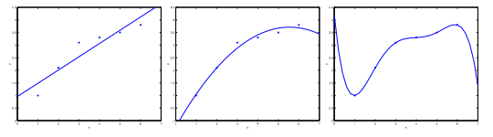
Instead, if we had added an extra feature \(x^2\), and fit \(y = \theta_0 + \theta_1x + \theta_2x^2\), then we obtain a slightly better fit to the data (see middle figure). Naively, it might seem that the more features we add, the better. However, there is also a danger in adding too many features: the rightmost figure is the result of fitting a 5th order polynomial. We see that even though the fitted curve passes through the data perfectly, we would not expect this to be a very good predictor of, say, housing prices (y) for different living areas (x). The left figure shows an instance of underfitting — in which the data clearly shows structure not captured by the model — and the figure on the right is an example of overfitting.
Underfitting, or high bias, is when the form of our hypothesis function h maps poorly to the tend of the data. It is usually caused by a function that is too simple or uses too few features. At the other extreme, overfitting, or high variance, is caused by a hypothesis function that fits the available data but does not generalize well to predict new data. It is usually caused by a complicated function that creates a lot of unnecessary curves and angles unrelated to the data. This terminology is applied to both linear and logistic regression.
There are two main options to address the issue of overfitting:
- Reduce the number of features:
- Manually select which features to keep
- Use a model selection algorithm (studied later in the course)
- Regularization
- Keep all the features, but reduce the magnitude of parameters \(\theta_j\).
- Regulaization works well when we have a lot of slightly useful features.
Cost Function
If we have overfitting from our hypothesis function, we can educe the weight that some of the terms in our function carry by increasing their cost.
Say we wanted to make the following function more quadratic:
\begin{equation} \theta_0 + \theta_1x + \theta_2x^2 + \theta_3x^3 + \theta_4x^4 \end{equation}We'll want to eliminate the influence of \(\theta_3x^3\) and \(\theta_4x^4\). Without actually getting rid of these features or changing the form of our hypothesis, we can instead modify our cost function:
\begin{equation} min_\theta \frac{1}{2m} \sum_{i=1}^{m} (h_\theta(x^{(i)}) - y^{(i)})^2 + 1000 \cdot \theta^2_3 + 100 \cdot \theta^2_4 \end{equation}We've added two extra terms at the end to inflate the cost of \(\theta_3\) and \(\theta_4\). Now, in order for the cost function to get close to zero, we will have to reduce the values of \(\theta_3\) and \(\theta_4\) to near zero. This will in turn greatly reduce the values of \(\theta_3x^3\) and \(\theta_4x^4\) in our hypothesis function.
We could also regularize all of our theta parameters in a single summation as:
\begin{equation} min_\theta \frac{1}{2m} \sum_{i=1}^{m} (h_\theta(x^{(i)}) - y^{(i)})^2 + \lambda \sum_{j=1}^{n} \theta^2_j \end{equation}The \(\lambda\) is the regulaization parameter. It determines how much the costs of our theta parametes are inflated.
Using the above cost function with the extra summation, we can smooth the output of our hypothesis function to reduce overfitting. If lambda is chosen to be too large, it may smooth out the function too much and cause underfitting.
Linear Regression and Logistic Regression
See the course for the algorithms and equations necessary for gradient descent and the normal equation.